Representation and Interpolation
by Suraj Rampure
Last modified: March 21, 2019
Previously, we discussed polynomials from a more combinatorial perspective. We will now transition to looking at polynomials in a more traditional light. We’ll start with a formal definition of what a polynomial is.
Definition
A polynomial is a function that consists solely of terms of the form $ax^k$, where $k$ is a non-negativeinteger, and $a$ is a real number. As a function, it takes real numbers as an input and returns real numbers as outputs ($f \colon \mathbb{R} \rightarrow \mathbb{R}$). More formally, we define an $n$th degree polynomial in the following way:
$\boxed{p(x) = \sum_{k = 0}^{n} a_kx^k = a_0 + a_1x + a_2x^2 + … + a_nx^n}$
We say a polynomial has degree $n$ if $x^{n}$ is the largest power of $x$ that has a non-zero coefficent, i.e.
$\textbf{deg}\left( p(x) \right) = \max_{k} \left(a_k \neq 0\right)$
$x-5$, $13x^{2} - 4x + 3$, $x^{14} + x^{13} + x^{4}$ and $4$ are all examples of polynomials, of degrees 1, 2, 14 and 0, respectively. Furthermore, these are all polynomials written in standard form – that is, the form defined above. We will look at different representations of polynomials shortly.
The degree of a polynomial defines several of its key features.
Point Representation
The first key feature is that a polynomial of degree $n$ is uniquely determined by a set of $n+1$ points. This is a concept you may be familiar with, in regards to a line – given any two points in the Cartesian plane, there is exactly one line (i.e. a polynomial of degree 1) that passes through these points. It’s impossible to draw a different line that also passes through these two points. However, given just one point in the plane, there is an infinite number of points that pass through it.
This applies of polynomials of all degrees. Any three points uniquely determine a parabola (a polynomial of degree 2), however given any two or fewer points, an infinite number of parabolas pass through them.
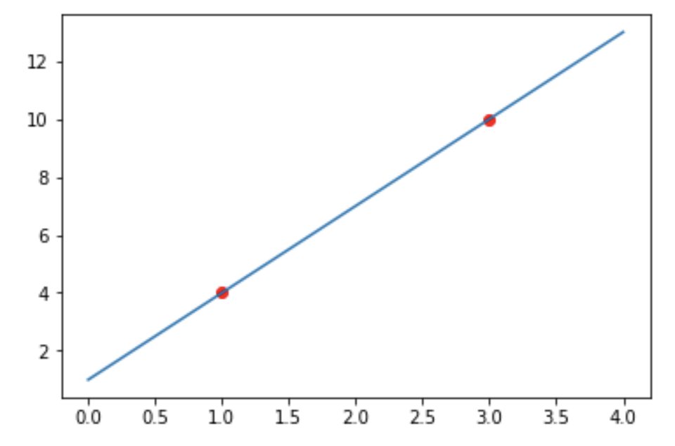
Here, we see the only linear polynomial that passes through the set of points $\{(1, 4), (3, 10)\}$:
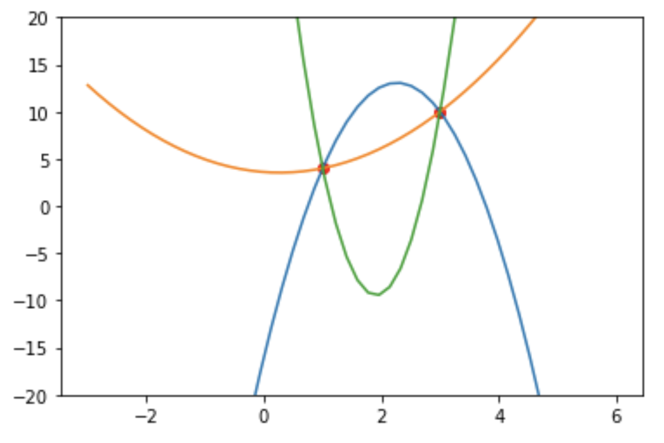
However, there are infinitely many parabolas that pass through these two points. Three of them are shown below:
Consider the set of points $S = \{(1, 3), (3, 19), (4, 33)\}$. These three points uniquely determine a degree 2 polynomial - you should verify on your own that this polynomial is $p(x) = 2x^2 + 1$. Since $2x^2 + 1$ is the only polynomial of degree 2 that passes through these points exactly, the set of points $S$ is an equivalent way of representing $p(x)$. We call this the point representation of polynomials.
We can easily convert between standard form and the point representation - given some degree $n$ polynomial, we can plug in $n+1$ points into it and record the $n+1$ pairs $(x_i, y_i)$ and call this our point representation. The question you may be asking, though, is how can we do the opposite - how can we find the standard form of a polynomial given the point representation, without repeated guessing and checking? How can we find that $p(x) = 2x^2 + 1$ is the polynomial defined by $S$? This process is called interpolation, and we will cover it now.
Interpolation
The question we’re now investigating is, given a set of $n+1$ points, how can we find the degree $n$ polynomial that uniquely interpolates it?
Odds are, you’ve seen the degree 1 case before. Given two points $(x_1, y_1)$ and $(x_2, y_2)$, we find the slope of the line passing through the points as $m = \frac{\Delta y}{\Delta x} = \frac{y_2 - y_1}{x_2 - x_1}$. We then substitute $m$ and either of the two given points into $y = mx + b$ to solve for $b$, giving us both coefficients. We need something more general, though, and there’s no natural extension to this process.
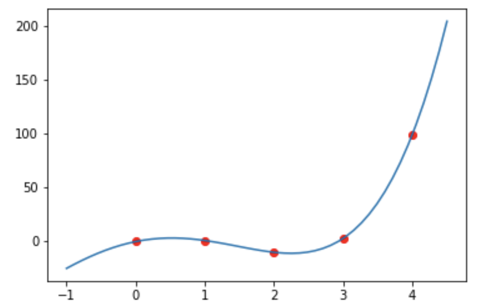
Suppose we’re given five points, $(0, -1), (1, 0), (2, -11), (3, 2)$ and $(4, 99)$. Since we know that we’re searching for a degree 4 polynomial, we could create $p(x) = ax^4 + bx^3 + cx^2 + dx + e$. Substituting each of the five points into $p(x)$ would give us a solvable system of 5 equations and 5 unknowns. These equations would be as follows:
$a(0)^4 + b(0)^3 + c(0)^2 + d(0) + e = -1\\a(1)^4 + b(1)^3 + c(1)^2 + d(1) + e = 0\\a(2)^4 + b(2)^3 + c(2)^2 + d(2) + e = -11\\a(3)^4 + b(3)^3 + c(3)^2 + d(3) + e = 2\\a(4)^4 + b(4)^3 + c(4)^2 + d(4) + e = 99$
However, solving this system of equations and unknowns would take quite some time. Luckily, there exists a more intuitive way to construct $p(x)$. Since there is only one such degree 4 polynomial that passes through these five points, both methods should (and do) result in the same $p(x)$.
Lagrange Interpolation
Instead of trying to create $p(x)$ at once, let’s try and create five smaller polynomials, that we can then sum to create $p(x)$. For each provided point $(x_i, y_i)$, $(x_1, y_1)$ being the first point we were given, we want to craft a sub-polynomial $p_{i}$ with the following properties:
-
$p_i(x_i) = 1$
-
$p_i(x_j) = 0, \forall \: j \neq i$
In other words, sub-polynomial $i$ should evaluate to 1 if $x_i$ is passed in, and to 0 if any of the other four $x_j$s are passed in (we will see why this structure is important very soon). We can create such a sub-polynomial, for each $i$, as follows:
For clarity, let’s calculate $p_1(x)$ and $p_3(x)$ (corresponding to $(0, 16)$ and $(2, -2)$, respectively, as these were the first and third points given to us).
$ p_3(x) = \frac{\Pi_{j \neq 3}(x - x_j)}{\Pi_{j \neq 3}(0 - x_j)} = \frac{(x-0)(x-1)(x-3)(x-4)}{(2-0)(2-1)(2-3)(2-4)} = \frac{1}{4}(x)(x-1)(x-3)(x-4) $
The second-to-last step of the above expansions best illustrate why we’ve chosen to craft our sub-polynomials in this way; if we were to evaluate $p_1(0)$, the numerator and denominator would be exactly the same. If we were to instead evaluate $p_1(1), p_1(2), p_1(3)$ or $p_1(4)$, since $x-1, x-2, x-3, x-4$ are all factors of the numerator the result would be 0.
We’re almost done. We can now say that our final polynomial $p(x)$ is constructed as follows:
This is where the $y$ values of each of the given points come into play. Looking at our example more closely, we have:
From the way each $p_i(x)$ was constructed, $p(0) = (-1) \cdot 1 + 0 \cdot 0 + (-11) \cdot 0 + 2 \cdot 0 + 99 \cdot 0 = -1$, and so on and so forth, as we expected. Doing the arithmetic yields the original polynomial, $p(x) = x^4 - 13x^2 + 13x - 1$.
This entire process is known as Lagrange Interpolation. It is named after Lagrange, a famous French mathematician. Lagrange Interpolation is still tedious, though not nearly as tedious as the initial approach from the start of this section. You should practice this process on your own; create your own polynomial of degree $n \leq 5$, pick $n+1$ points on it, and see if you can correctly reconstruct your polynomial.
It should be noted though, that mastering the arithmetic, while important, isn’t the goal of learning this material. This material is presented so that you can add it to your mathematical toolbox.